Bayesian Machine Learning & Probabilistic AI

Bayesian Machine Learning & Probabilistic AI

Bayesian inference, Uncertainty estimation

Introduction

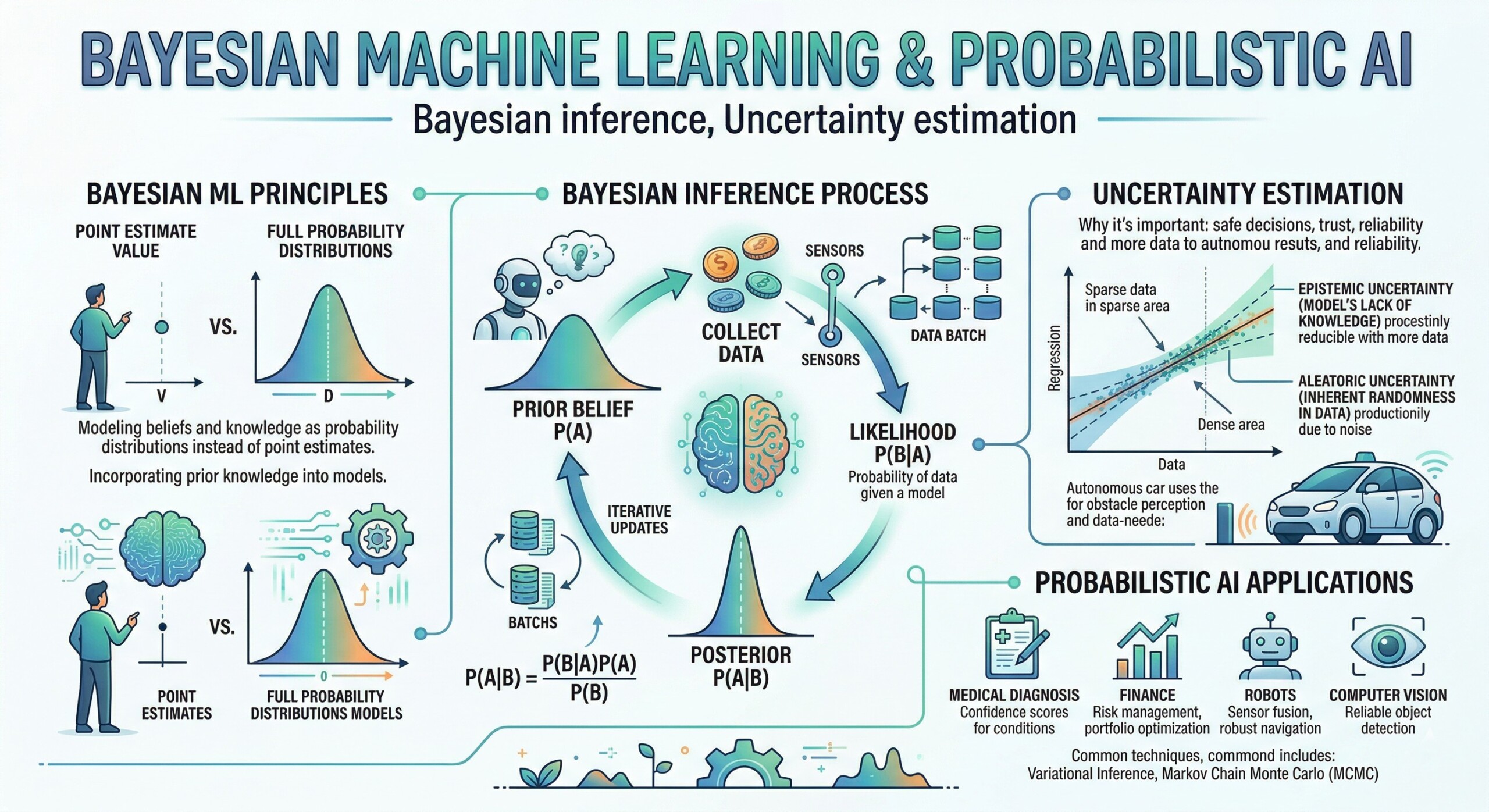
In the evolving landscape of artificial intelligence, one of the most powerful shifts has been from deterministic models to probabilistic thinking. Traditional machine learning models often provide single-point predictions – clear, decisive outputs that mask the uncertainty inherent in real-world data. However, the real world is rarely certain. Data is noisy, incomplete, and dynamic. This is where Bayesian Machine Learning and Probabilistic AI emerge as transformative paradigms, enabling systems not just to predict, but to reason under uncertainty.

At the heart of Bayesian thinking lies a simple yet profound idea: beliefs should be updated as new evidence becomes available. Instead of treating model parameters as fixed values, Bayesian methods treat them as probability distributions. This allows models to express degrees of confidence in their predictions, making them particularly valuable in high-stakes domains such as healthcare, finance, and autonomous systems. The result is a more transparent, interpretable, and robust form of AI.

Probabilistic AI extends this philosophy further by embedding uncertainty directly into the modeling process. It integrates principles from probability theory, statistics, and machine learning to create systems that can quantify ambiguity, learn from limited data, and adapt over time. In an era where trust in AI systems is critical, Bayesian approaches provide a principled framework for building systems that are not only intelligent but also reliable and accountable.

Let’s dive deep into the topic.

1. Bayesian Inference: Updating Beliefs with Data

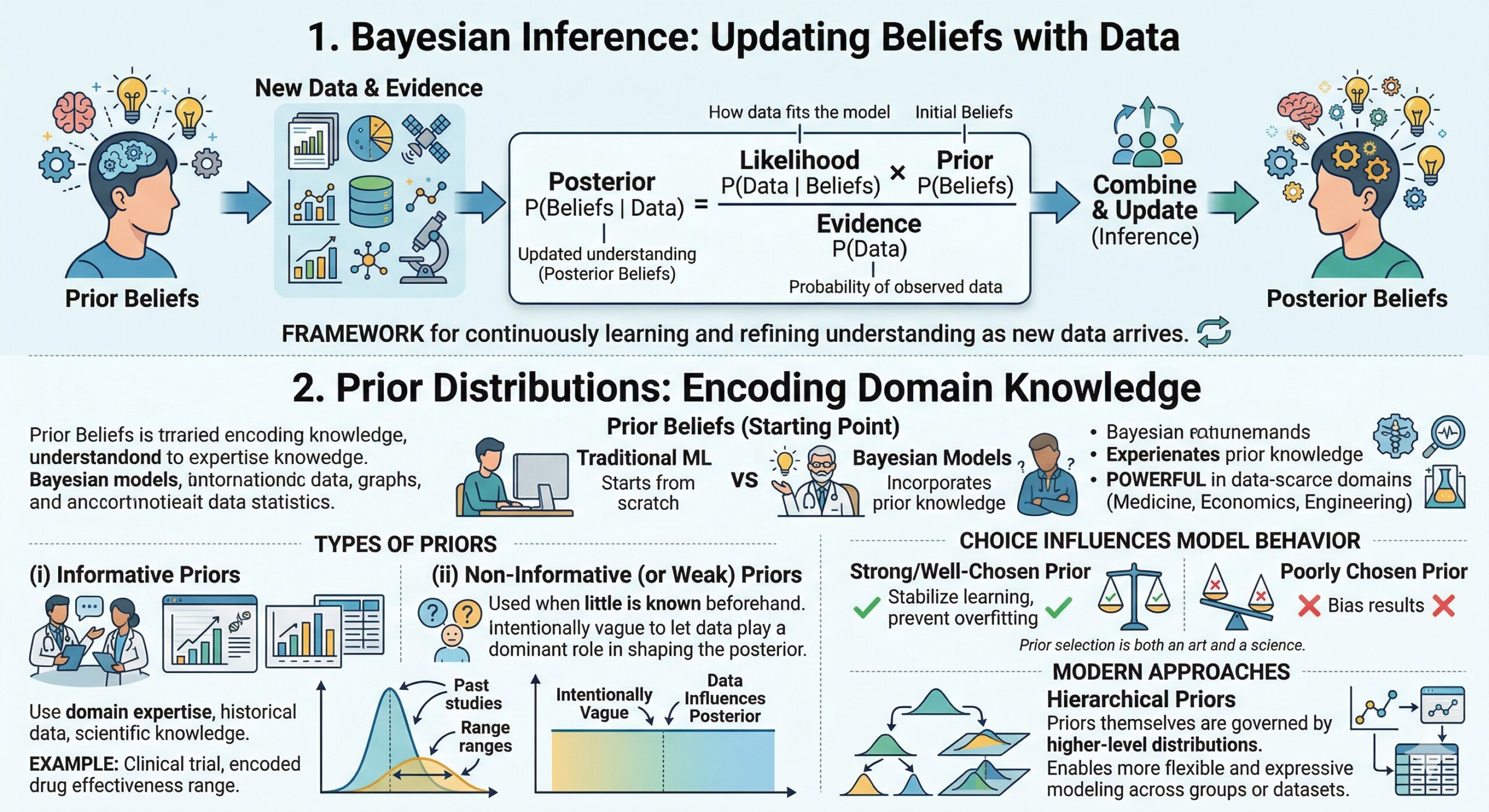
Bayesian inference is grounded in the idea of updating prior beliefs with observed data to obtain posterior beliefs. It is mathematically expressed as:

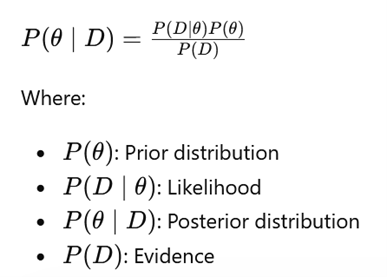
This framework allows models to continuously learn and refine their understanding as new data arrives.

2. Prior Distributions: Encoding Domain Knowledge

Priors are the starting point of Bayesian inference and represent what we believe about a system before observing any data. Unlike traditional machine learning models that start from scratch, Bayesian models can incorporate prior knowledge – making them especially powerful in domains where data is scarce but expertise is rich, such as medicine, economics, or engineering.

There are broadly two types of priors.

(i) Informative priors are constructed using domain expertise, historical data, or scientific knowledge. For example, in a clinical trial, prior studies may suggest that a drug has a certain effectiveness range, and this can be encoded into the model.

(ii) On the other hand, non-informative (or weak) priors are used when little is known beforehand. These priors are intentionally vague so that the data plays a dominant role in shaping the posterior.

The choice of prior is not merely a technical detail – it fundamentally influences the model’s behaviour, especially when data is limited. A strong prior can stabilize learning and prevent overfitting, while a poorly chosen prior can bias results. This makes prior selection both an art and a science. Modern approaches also use hierarchical priors, where priors themselves are governed by higher-level distributions, enabling more flexible and expressive modeling across groups or datasets. An excellent collection of learning videos awaits you on our Youtube channel.

3. Likelihood Function: Connecting Model to Data

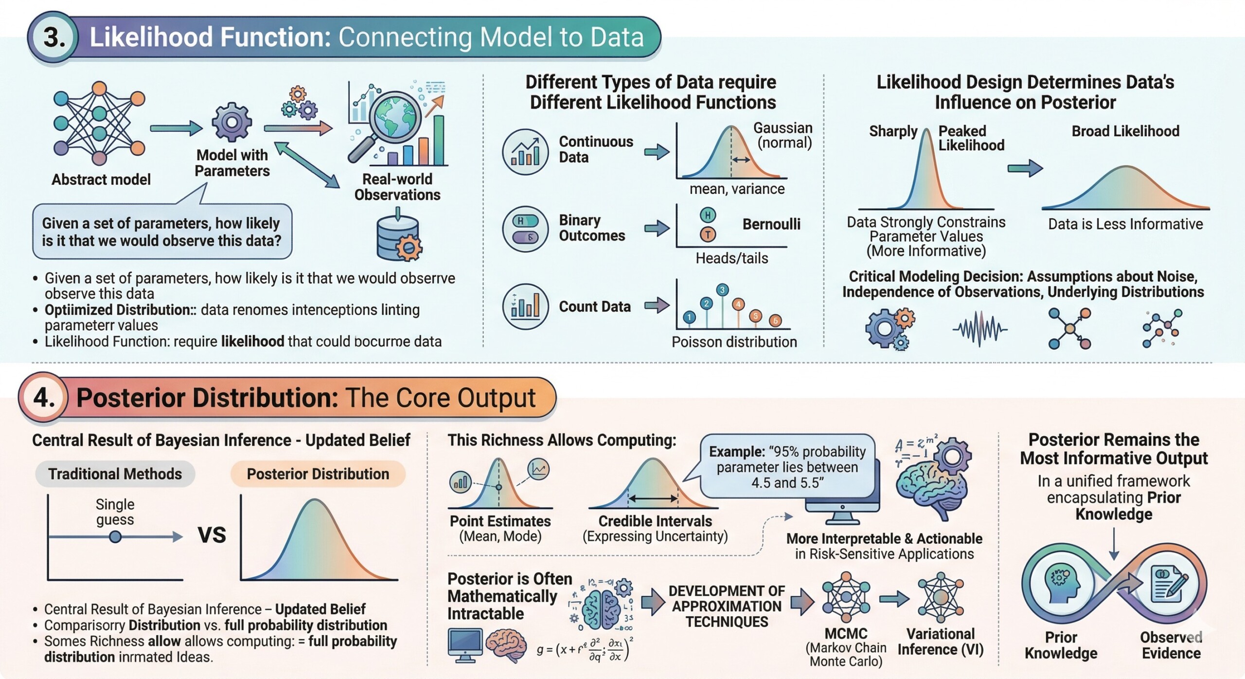
The likelihood function defines how the observed data relates to the model parameters. It answers the question: Given a set of parameters, how likely is it that we would observe this data? This component is crucial because it anchors the abstract model to real-world observations.

Different types of data require different likelihood functions. For continuous data, a Gaussian (normal) likelihood is often used, assuming that observations are centered around a mean with some variance. For binary outcomes, a Bernoulli likelihood is appropriate, while count data might use a Poisson distribution. Choosing the correct likelihood ensures that the model accurately reflects the data-generating process.

Moreover, the likelihood function plays a key role in determining how strongly the data influences the posterior. If the likelihood is sharply peaked, it means the data strongly constrains the parameter values. If it is broad, the data is less informative. In practice, likelihood design also involves assumptions about noise, independence of observations, and underlying distributions – making it a critical modeling decision that directly impacts performance and interpretability.

4. Posterior Distribution: The Core Output

The posterior distribution is the central result of Bayesian inference – it represents the updated belief about the model parameters after observing data. Unlike traditional methods that yield a single “best” estimate, the posterior provides a full probability distribution, capturing all plausible parameter values and their associated probabilities.

This richness allows practitioners to compute not just point estimates (like the mean or mode), but also credible intervals, which express uncertainty in a principled way. For example, instead of saying “the parameter is 5,” a Bayesian model might say “there is a 95% probability that the parameter lies between 4.5 and 5.5.” This makes the results more interpretable and actionable, especially in risk-sensitive applications.

However, computing the posterior is often mathematically intractable, especially for complex models. This has led to the development of approximation techniques such as MCMC and variational inference. Despite these challenges, the posterior remains the most informative output of a Bayesian model, as it encapsulates both prior knowledge and observed evidence in a unified framework. A constantly updated Whatsapp channel awaits your participation.

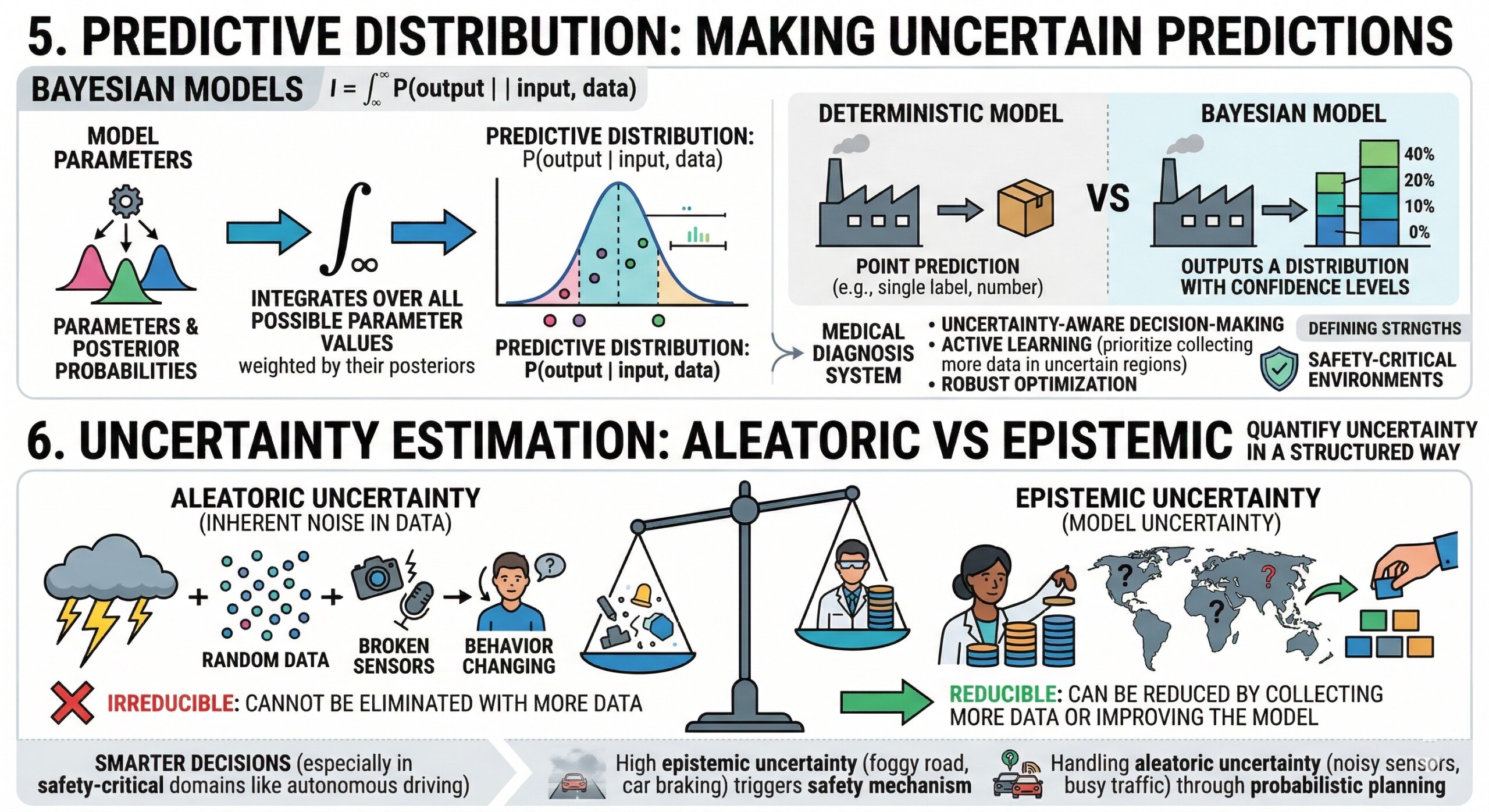
5. Predictive Distribution: Making uncertain predictions

Instead of predicting a single output, Bayesian models compute a predictive distribution:

This integrates over all possible parameter values, resulting in predictions that naturally incorporate uncertainty.

In Bayesian machine learning, predictions are not single values but distributions. The predictive distribution integrates over all possible parameter values, weighted by their posterior probabilities. This results in predictions that inherently account for uncertainty in both the data and the model.

This approach contrasts sharply with deterministic models, which provide point predictions without any indication of confidence. For instance, in a medical diagnosis system, a Bayesian model might output a probability distribution over possible diseases, along with confidence levels, rather than a single definitive label. This is invaluable for decision-making, as it allows practitioners to assess risk and consider alternative outcomes.

Predictive distributions also enable advanced capabilities such as uncertainty-aware decision-making, active learning, and robust optimization. For example, a system can choose to defer decisions when uncertainty is high or prioritize collecting more data in uncertain regions. This makes Bayesian models particularly suited for real-world environments where uncertainty is unavoidable and must be explicitly managed.

6. Uncertainty Estimation: Aleatoric vs Epistemic

Bayesian methods distinguish between:

• Aleatoric uncertainty: Inherent noise in data (irreducible)
• Epistemic uncertainty: Model uncertainty due to limited data (reducible)

This distinction is critical for decision-making, especially in safety-critical applications.

So a defining strength of Bayesian methods is their ability to quantify uncertainty in a structured way. Understanding this distinction is critical for building reliable AI systems.

Aleatoric uncertainty arises from inherent randomness or noise in the data. For example, sensor noise in a camera or variability in human behaviour cannot be eliminated, no matter how much data is collected. This type of uncertainty is irreducible and must be modeled explicitly to avoid overconfidence.

Epistemic uncertainty, on the other hand, stems from a lack of knowledge. It occurs when the model has not seen enough data or encounters unfamiliar scenarios. Unlike aleatoric uncertainty, epistemic uncertainty can be reduced by collecting more data or improving the model. Bayesian methods naturally capture this by maintaining distributions over parameters.

Distinguishing between these two types allows systems to make smarter decisions. For instance, in autonomous driving, high epistemic uncertainty might trigger a safety mechanism, while aleatoric uncertainty might be handled through probabilistic planning. This nuanced understanding of uncertainty is one of the key reasons Bayesian AI is gaining traction in safety-critical domains. Excellent individualised mentoring programmes available.

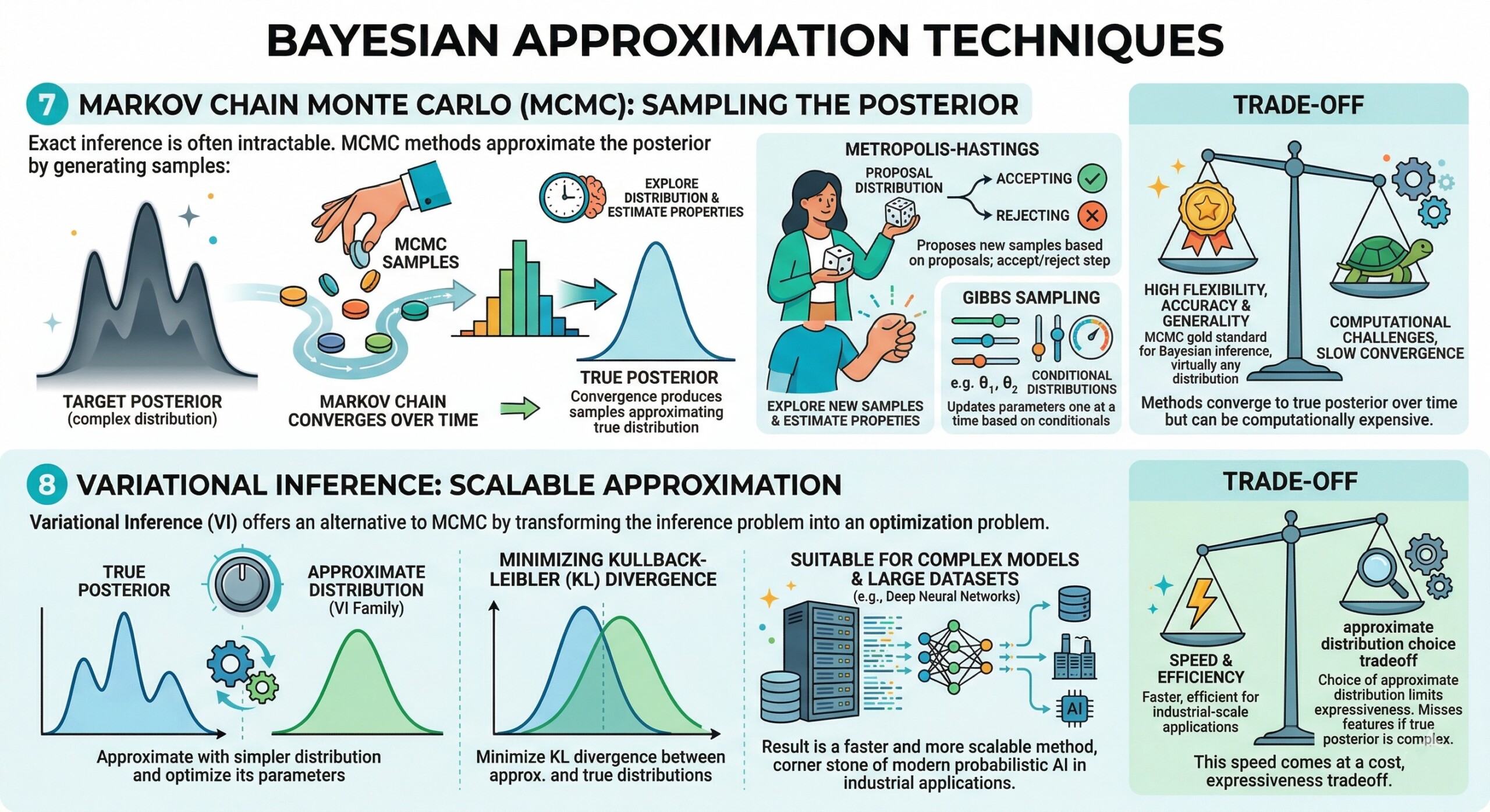
7. Markov Chain Monte Carlo (MCMC): Sampling the Posterior

Exact inference is often intractable. MCMC methods approximate the posterior by generating samples:

• Metropolis-Hastings
• Gibbs Sampling

These methods converge to the true posterior over time but can be computationally expensive.

MCMC methods are a class of algorithms used to approximate complex posterior distributions by generating samples. Since exact computation of the posterior is often infeasible, MCMC provides a practical way to explore the distribution and estimate its properties.

The core idea is to construct a Markov chain whose stationary distribution is the target posterior. Over time, the chain produces samples that approximate the true distribution. Popular algorithms include Metropolis-Hastings, which proposes new samples based on a proposal distribution, and Gibbs Sampling, which updates parameters one at a time based on conditional distributions.

While MCMC is highly flexible and can approximate virtually any distribution, it comes with computational challenges. Convergence can be slow, especially in high-dimensional spaces, and diagnosing whether the chain has converged is non-trivial. Despite these limitations, MCMC remains a gold standard for Bayesian inference due to its accuracy and generality.

8. Variational Inference: Scalable Approximation

Variational Inference (VI) offers an alternative to MCMC by transforming the inference problem into an optimization problem. Instead of sampling from the posterior, VI approximates it with a simpler distribution and optimizes the parameters of this distribution to be as close as possible to the true posterior.

This is typically done by minimizing the Kullback-Leibler (KL) divergence between the approximate and true distributions. The result is a faster and more scalable method, making it suitable for large datasets and complex models such as deep neural networks.

However, this speed comes at a cost. The choice of the approximate distribution (often called the variational family) can limit the expressiveness of the model. If the true posterior is highly complex, the approximation may miss important features. Despite this trade-off, VI has become a cornerstone of modern probabilistic AI, especially in industrial-scale applications where computational efficiency is critical. Subscribe to our free AI newsletter now.

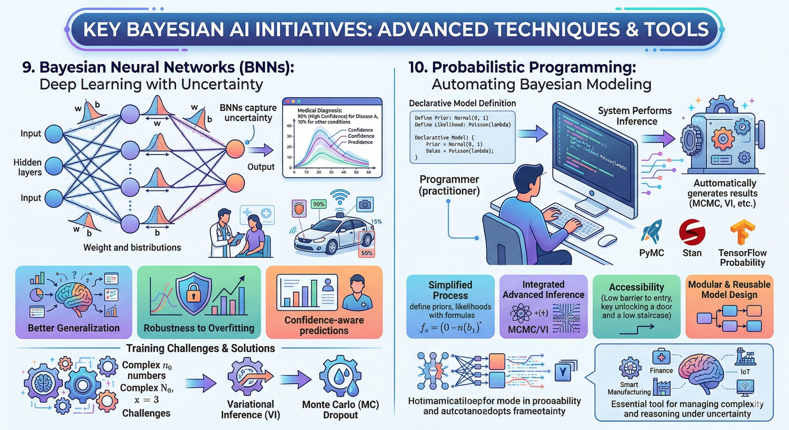
9. Bayesian Neural Networks (BNNs): Deep Learning with Uncertainty

BNNs extend neural networks by placing distributions over weights instead of fixed values. This enables:

• Confidence-aware predictions
• Better generalization
• Robustness to overfitting

They are increasingly used in applications like medical diagnosis and autonomous driving.

Bayesian Neural Networks extend traditional neural networks by placing probability distributions over their weights and biases. Instead of learning fixed parameters, BNNs learn distributions, allowing them to capture uncertainty in both the model and its predictions.

This has several advantages. First, BNNs provide confidence estimates alongside predictions, which is crucial for applications like medical diagnosis or financial forecasting. Second, they are more robust to overfitting, as the distribution over weights acts as a form of regularization. Third, they can better handle out-of-distribution data by expressing higher uncertainty when encountering unfamiliar inputs.

Training BNNs is computationally challenging due to the need to approximate posterior distributions over potentially millions of parameters. Techniques such as variational inference and Monte Carlo dropout are often used to make training tractable. Despite these challenges, BNNs represent a powerful fusion of deep learning and probabilistic modeling, pushing the boundaries of what AI systems can achieve.

10. Probabilistic Programming: Automating Bayesian Modeling

Frameworks like:

• PyMC
• Stan
• TensorFlow Probability

allow practitioners to define probabilistic models declaratively and perform inference automatically, democratizing access to Bayesian techniques.

Probabilistic programming languages (PPLs) are designed to simplify the process of building and training Bayesian models. Instead of manually deriving inference algorithms, practitioners can define models in a high-level, declarative way, and the system automatically performs inference.

Popular frameworks such as PyMC, Stan, and TensorFlow Probability provide tools for specifying priors, likelihoods, and model structures. They also integrate advanced inference algorithms like MCMC and variational inference, allowing users to focus on modeling rather than computation.

One of the key advantages of probabilistic programming is accessibility. It lowers the barrier to entry for Bayesian methods, enabling a broader range of practitioners to use them effectively. Additionally, PPLs support modular and reusable model design, making it easier to experiment with different assumptions and structures.

As AI systems become more complex, probabilistic programming is likely to play a central role in managing this complexity. It provides a unified framework for reasoning under uncertainty, making it an essential tool in the toolkit of modern AI practitioners. Upgrade your AI-readiness with our masterclass.

Conclusion

Bayesian Machine Learning represents a fundamental shift in how we think about intelligence in machines. Rather than striving for absolute certainty, it embraces ambiguity and models it explicitly. This shift is not merely technical – it is philosophical. It aligns AI systems more closely with human reasoning, where beliefs are constantly updated in light of new evidence, and uncertainty is an integral part of decision-making.

In practical terms, Bayesian approaches enable more robust, interpretable, and trustworthy AI systems. They provide a structured way to incorporate prior knowledge, handle limited data, and quantify confidence in predictions. As AI systems become more embedded in critical aspects of society, from healthcare diagnostics to financial risk assessment, the ability to reason under uncertainty becomes not just desirable, but essential.

Looking ahead, the integration of Bayesian methods with deep learning and large-scale AI systems will likely define the next frontier of intelligent systems. Probabilistic AI is not just an alternative approach—it is a necessary evolution toward building AI that is not only powerful but also transparent, accountable, and aligned with real-world complexity.