Optimization Landscapes in Deep Learning

Optimization Landscapes in Deep Learning
Loss surfaces, saddle points; Sharp vs flat minima
Introduction
Deep learning models have achieved remarkable success across domains, from computer vision to natural language processing. Beneath this success lies a complex mathematical challenge called optimization. Training a neural network means navigating a high dimensional landscape defined by its loss function.
This landscape, often called the loss surface or optimization landscape, is not smooth or simple. It contains hills, valleys, plateaus, and flat regions that can slow or mislead the training process. Understanding this terrain is essential because it directly affects how well a model learns and performs on unseen data.
Unlike classical optimization problems, deep learning involves millions or even billions of parameters. This creates extremely high dimensional spaces where unusual phenomena such as saddle points, sharp minima, and flat minima emerge. These behave very differently from what we see in low dimensional settings.
We now explore the geometry of these landscapes, the challenges they create, and how modern optimization techniques handle them effectively.
Let’s dive deep into the topic.
1. What is a ‘Loss Surface’
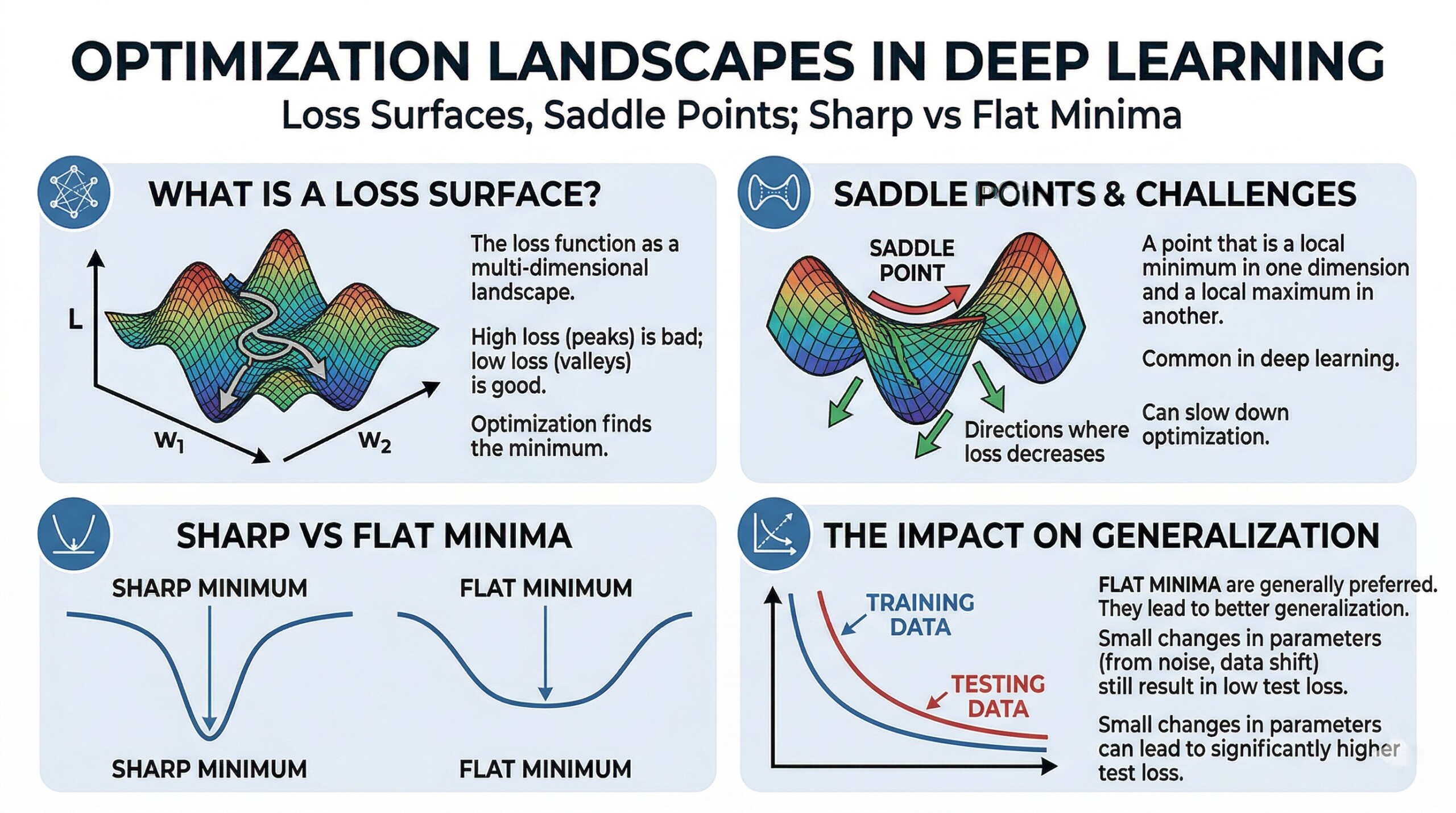
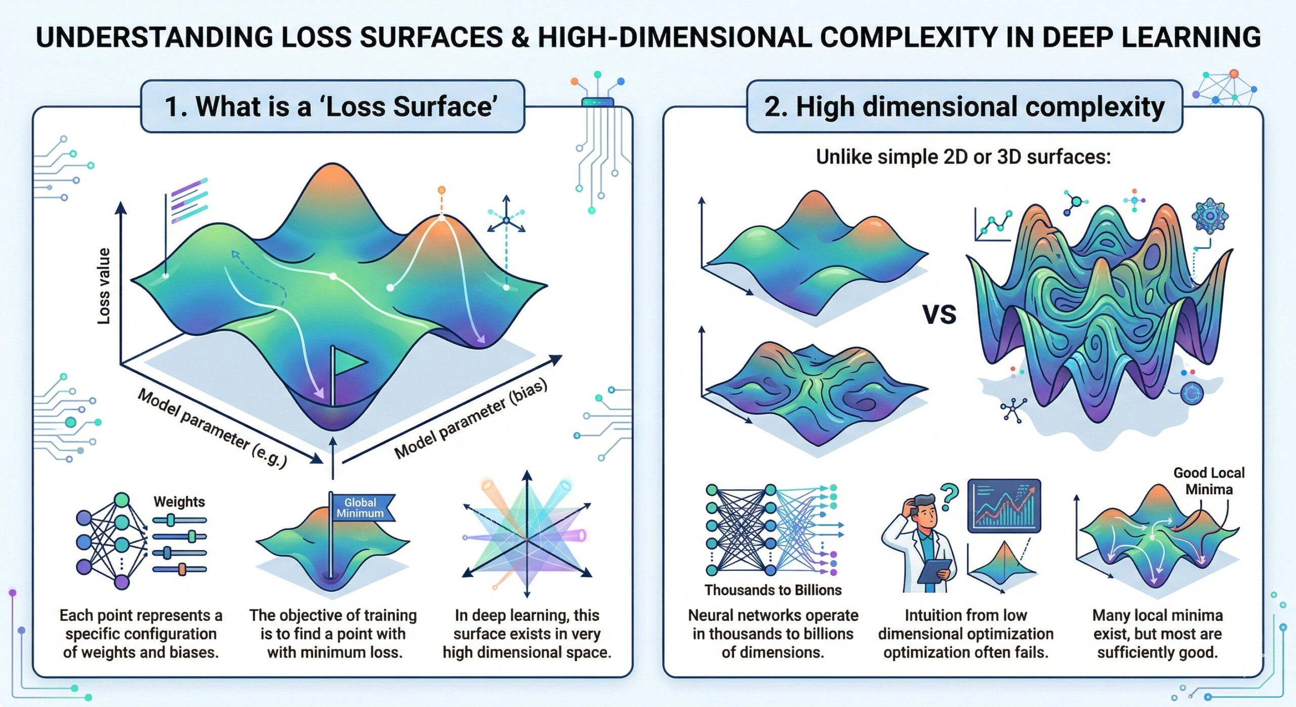
A loss surface is a mapping from model parameters to a scalar loss value.
- Each point represents a specific configuration of weights and biases.
- The objective of training is to find a point with minimum loss.
- In deep learning, this surface exists in very high dimensional space.
2. High dimensional complexity
Unlike simple 2D or 3D surfaces:
- Neural networks operate in thousands to billions of dimensions.
- Intuition from low dimensional optimization often fails.
- Many local minima exist, but most are sufficiently good. An excellent collection of learning videos awaits you on our Youtube channel.
3. Gradient Descent as navigation
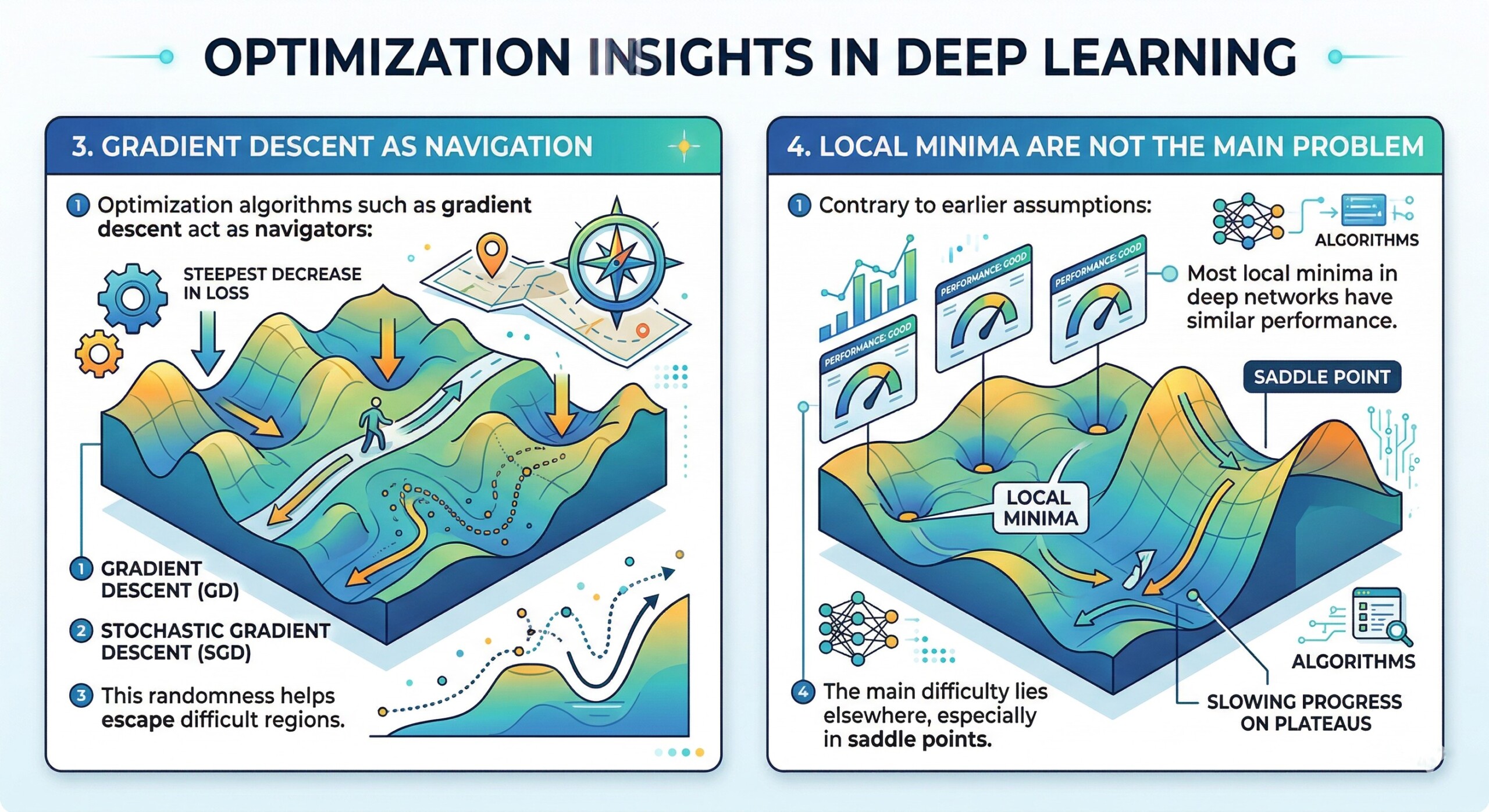
Optimization algorithms such as gradient descent act as navigators:
- They move in the direction of steepest decrease in loss.
- Stochastic Gradient Descent introduces randomness.
- This randomness helps escape difficult regions.
4. Local Minima are not the main problem
Contrary to earlier assumptions:
- Most local minima in deep networks have similar performance.
- The main difficulty lies elsewhere, especially in saddle points. A constantly updated Whatsapp channel awaits your participation.
5. Saddle Points as a key challenge
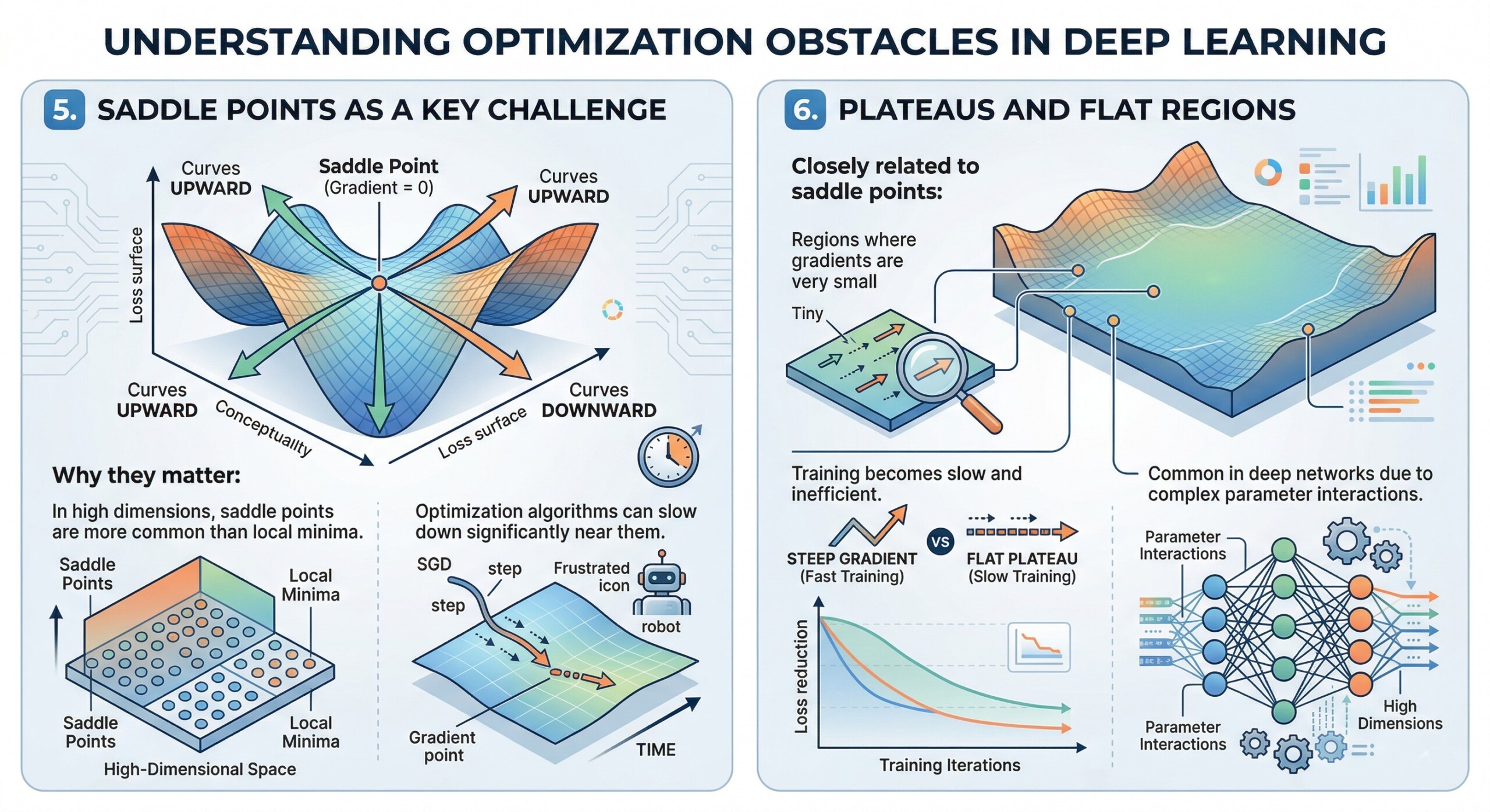
A saddle point is:
- A point where the gradient is zero but it is not a minimum.
- The surface curves upward in some directions and downward in others.
Why they matter:
- In high dimensions, saddle points are more common than local minima.
- Optimization algorithms can slow down significantly near them.
6. Plateaus and flat regions
Closely related to saddle points:
- Regions where gradients are very small.
- Training becomes slow and inefficient.
- Common in deep networks due to complex parameter interactions. Excellent individualised mentoring programmes available.
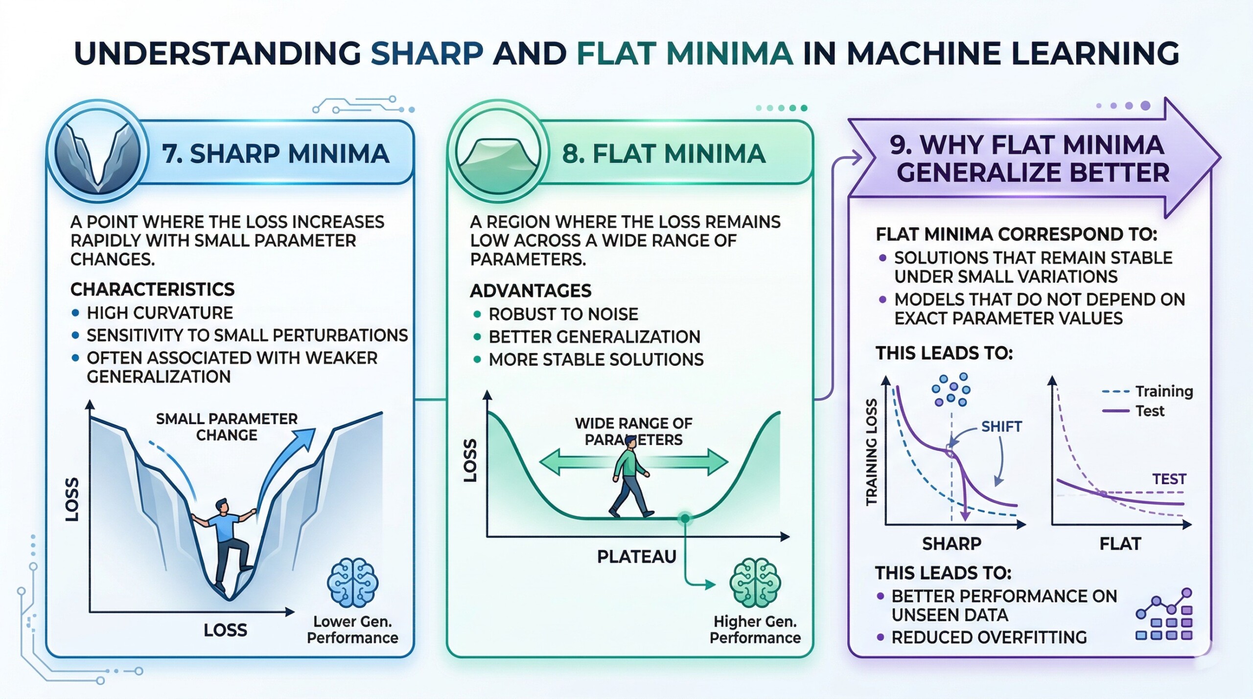
7. Sharp Minima
A sharp minimum is:
- A point where the loss increases rapidly with small parameter changes.
Characteristics:
- High curvature
- Sensitivity to small perturbations
- Often associated with weaker generalization
8. Flat Minima
A flat minimum is:
- A region where the loss remains low across a wide range of parameters.
Advantages:
- Robust to noise
- Better generalization
- More stable solutions. Subscribe to our free AI newsletter now.
9. Why Flat Minima generalize better
Flat minima correspond to:
- Solutions that remain stable under small variations
- Models that do not depend on exact parameter values
This leads to:
- Better performance on unseen data
- Reduced overfitting
10. Role of Optimization techniques
Modern methods help navigate the landscape:
- SGD with momentum helps move past saddle points
- Adaptive optimizers like Adam adjust learning rates
- Regularization techniques such as dropout and weight decay promote flatter minima
- Batch size influences whether sharp or flat minima are reached. Upgrade your AI-readiness with our masterclass.
Conclusion
The optimization landscape in deep learning is highly complex and fundamentally different from traditional optimization problems. Training a neural network involves navigating a high dimensional space filled with saddle points, flat regions, and minima with varying shapes.
A key insight from modern research is that not all minima are equally useful. While many parameter configurations may achieve low training loss, those located in flat regions of the loss surface tend to perform better on new data and remain more stable.
Saddle points, rather than local minima, represent a major challenge in high dimensional optimization. This has influenced the design of modern optimization algorithms, which use randomness, momentum, and adaptive strategies to move efficiently through the landscape.
Understanding these concepts is essential for designing effective models and training strategies. As deep learning systems continue to grow in scale and complexity, a deeper grasp of optimization landscapes becomes increasingly important for building models that are accurate, robust, and reliable.
Share this with the world
Related Articles
